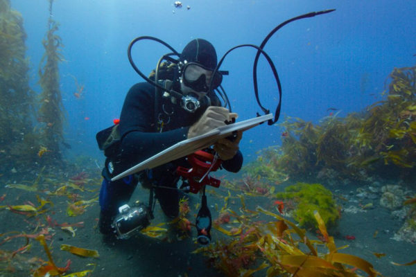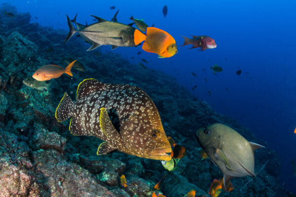
Revealing and protecting underwater worlds
Our Explorers discover, understand, and conserve marine and coastal systems and inspire and empower local and global audiences to better understand and protect the ocean.

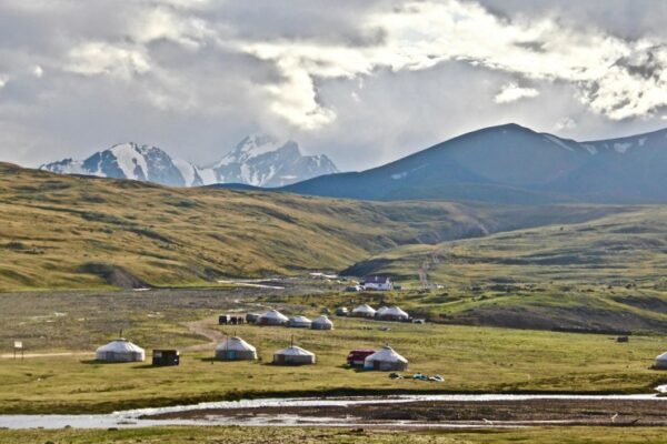
Preserving and protecting land environments
Our Explorers explore, understand, and conserve terrestrial and freshwater systems and inspire and empower local and global audiences to better understand and protect our lands, lakes, and rivers.

Protecting and conserving wildlife
Our Explorers inspire and empower local and global audiences to better understand and protect wildlife, including animals, plants and fungi.

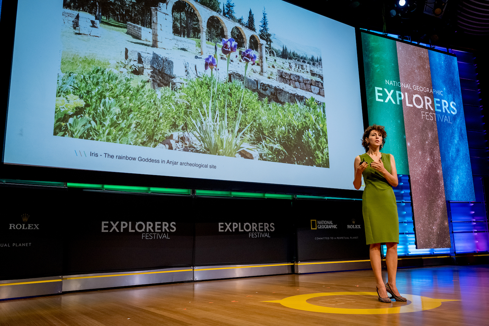
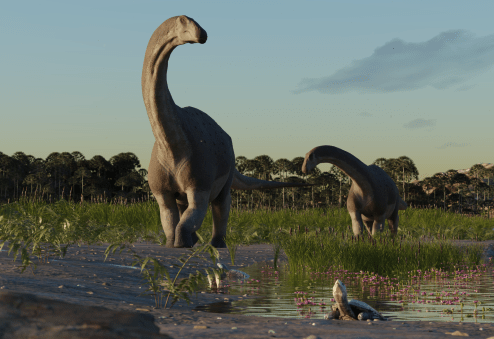
Understanding our past and protecting our future
Our Explorers work to preserve cultural knowledge, better understand human histories, cultures, practices, diversity, and evolution—past and present, center communities, and inform and inspire global audiences with stories or lessons about humanity.

Supporting innovation
Our Explorers are taking novel and inventive approaches to address critical challenges and produce insights that illuminate and protect the wonder of our world.